Extending Lee–Carter Models with inlabru: Spatio-Temporal Applications in Health and Mortality

Sara Martino

sara.martino@ntnu.no

Dept. of Mathematical Science, NTNU

Outline

• Motivation
• The Lee-Carter Model
• A Bayesian formulation of the Lee-Carter Model
• inlabru
• Cognitive impairment across USA
• Mortality in Italy
• Conclusion

Motivation

Spatio-Temporal trends in Health and Mortality

• Mortality in Italy across 107 provinces in 2002-2019
• Cognitive impairment across USA states from 2008-2022

How do these phenomena change across age, and how do patterns evolve over space and time?

What is common?

Both mortality and mental health have strong structure across age, time and space. The interaction between these effects cannot be ignored.

Spatio-Temporal trends in Health and Mortality

• Mortality in Italy across 107 provinces in 1999-2019
• Cognitive impairment across USA states from 2008-2022

What is different?

Mortality

• Registry data
• Complete and of good quality
• random variability given the small size of the territorial units.

Cognitive impairment

• Survey data
• Necessary to account for complex survey design

The Lee-Carter Model

The Lee–Carter Model

The Lee-Carter model (Lee and Carter, 1992) is a popular forecasting model in demography.

The basic Lee-Carter model in a Poisson setting is: \[\begin{aligned} Y_{xt} \mid \lambda_{xt} &\sim \text{Poisson}(E_{xt} \lambda_{xt})\\ \log(\lambda_{xt}) &= \alpha_x + \beta_x \kappa_t + \varepsilon_{xt} \end{aligned}\]

Parameters:

• \(\alpha_x\) is an average age profile
• \(\kappa_t\) represents mortality changes over time
• \(\beta_x\) determines the age specific change when \(\kappa_t\) changes
• \(\varepsilon_{xt}\) adjusts for overdispersion

Parameter interpretation - \(\alpha_x\)

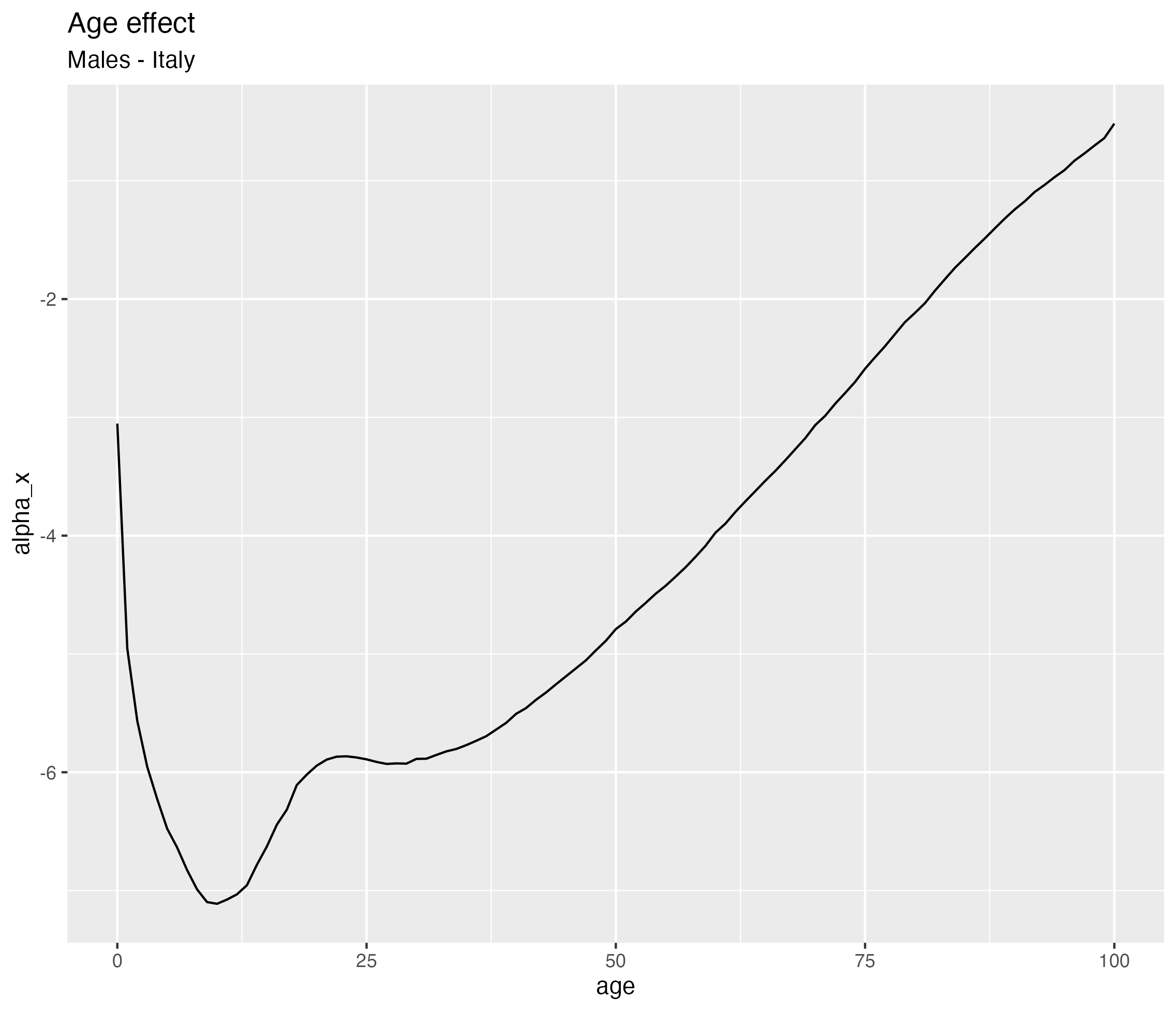
The basic Lee-Carter model \[\log(\lambda_{xt}) = \color{red}{\alpha_x} + \beta_x \kappa_t + \varepsilon_{xt}\]

• Average log-mortality at each age

• Captures:

  • high mortality at very young ages
    
  • low mortality in young adults
    
  • increasing mortality at older ages

👉 “what mortality looks like across ages in a typical year”

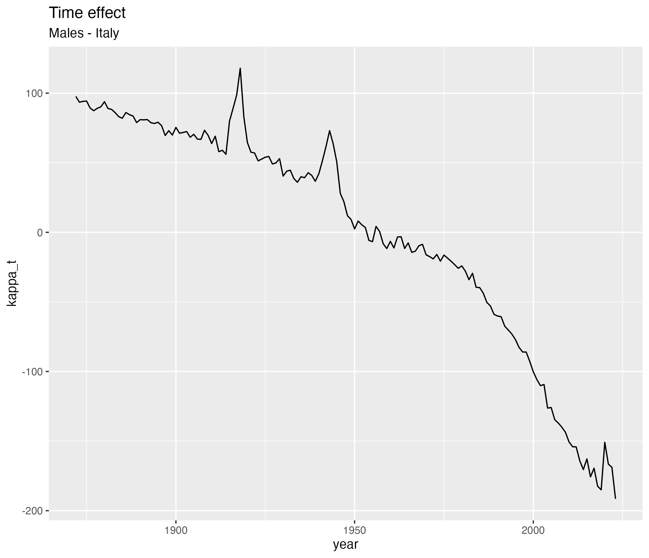
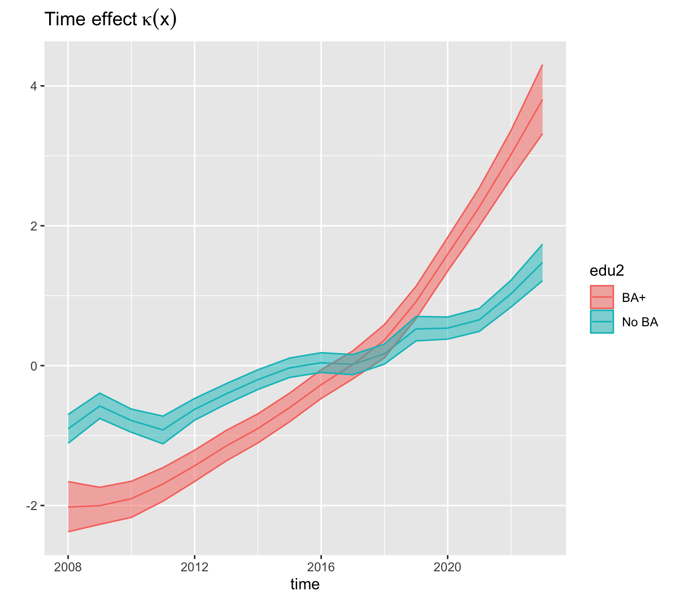
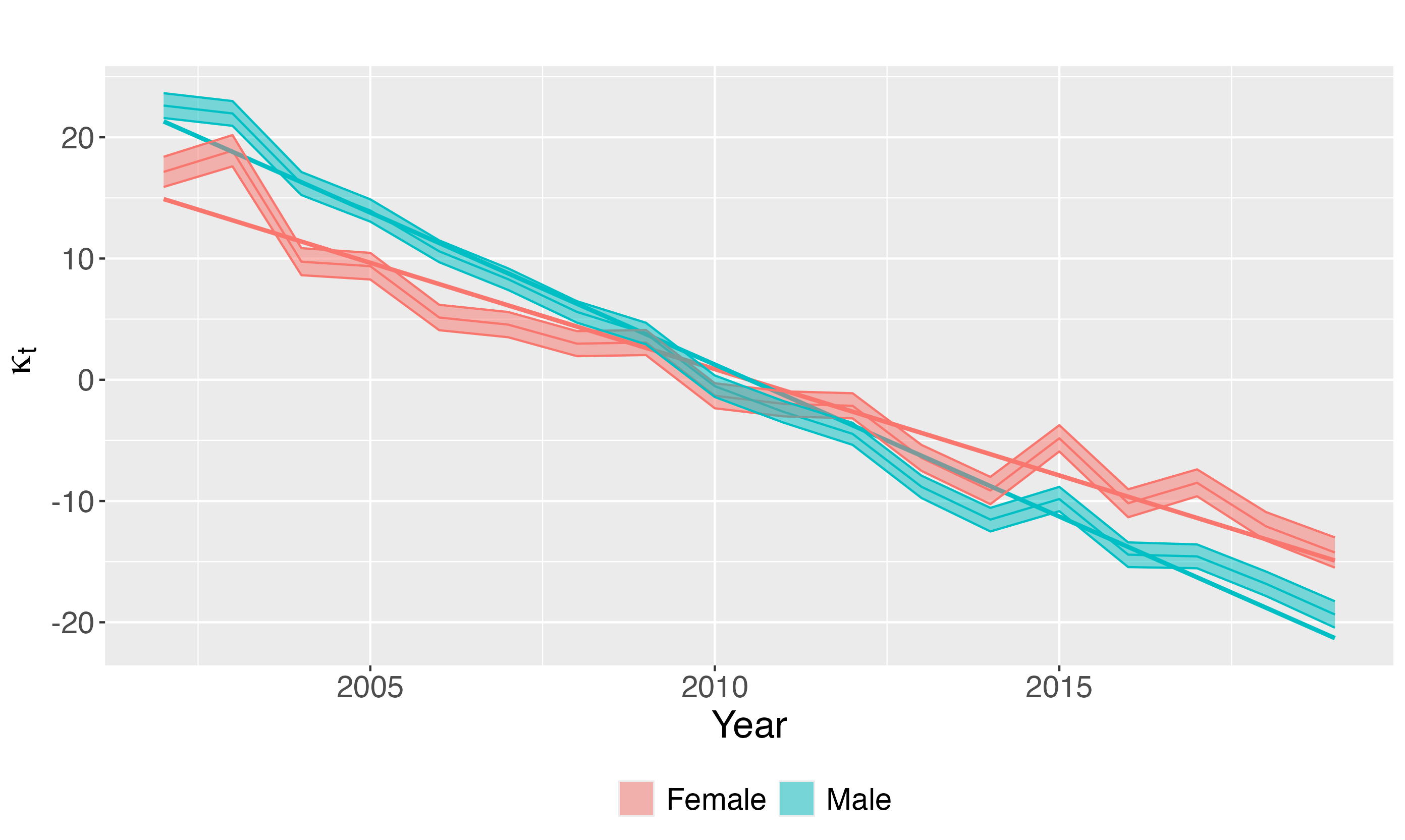
Parameter interpretation - \(\kappa_t\)

The basic Lee-Carter model \[\log(\lambda_{xt}) = \alpha_x + \beta_x\ \color{red}{\kappa_t} + \varepsilon_{xt}\]

• Captures:
  • overall improvements in mortality
    
  • medical progress
    
  • public health changes

👉 “the overall level of mortality in a given year”

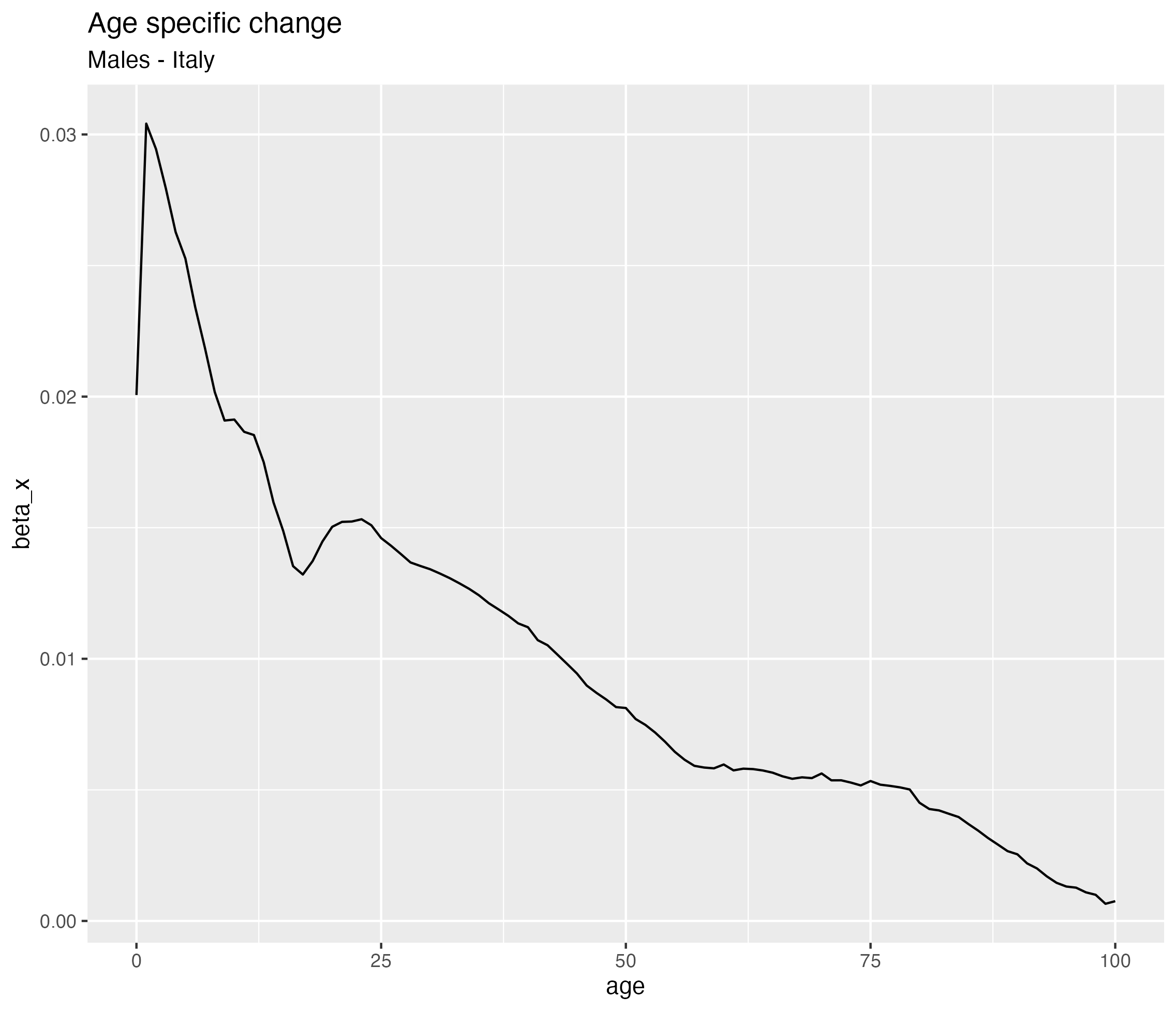
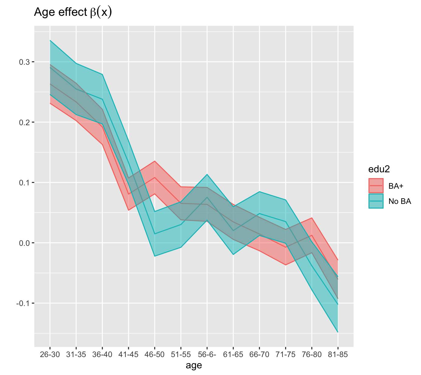
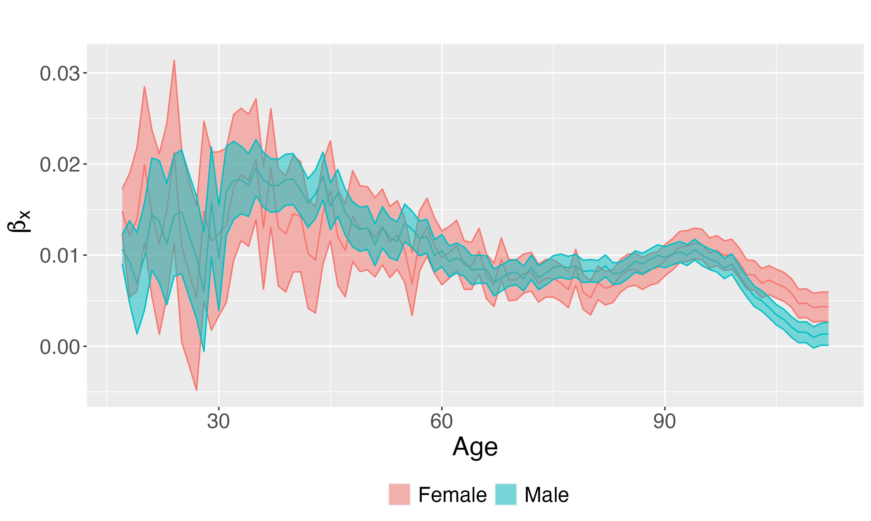
Parameter interpretation - \(\beta_t\)

The basic Lee-Carter model \[\log(\lambda_{xt}) = \alpha_x + \color{red}{\beta_x}\ \kappa_t + \varepsilon_{xt}\]

• Measures how each age reacts to changes in \(\kappa_t\)

• If:

  • \(\beta_x\) large → mortality at age \(x\) changes a lot
    
  • \(\beta_x\) small → little change over time

👉 “which ages benefit most from progress”

Identifiability Constraints

Model is not unique:

\[\alpha_x + \beta_x \kappa_t = \alpha_x + (c \beta_x)(\kappa_t / c)\]

So we impose constraints:

• \(\sum_t \kappa_t = 0\)
• \(\sum_x \beta_x = 1\)

👉 Ensures unique interpretation of parameters

Inference for Lee-Carter Model

The Lee-Carter model has classically been estimated in a frequentist setting using a singular value decomposition (SVD).

The R-packages demography, ilc or StoMoMo can be used to implement the original Lee-Carter model and some of its extensions.

How about Bayesian Inference?

Czado et al (2005) proposed to place the Lee-Carter model in a Bayesian framework. Wiśniowski et al. (2015) use MCMC.

How about INLA?

A Bayesian formulation of the Lee-Carter Model

Bayesian version of the Poisson Lee-Carter model

\[\begin{align*} Y_{xt} \mid \lambda_{xt} &\sim \text{Poisson}(E_{xt} \lambda_{xt})\ \log(\lambda_{xt}) &= \alpha_x + \beta_x \kappa_t + \epsilon_{xt} \end{align*}\] with

• \(\alpha_x \mid \tau_\alpha \sim \mathcal{N}(0, \tau_\alpha)\), for \(x=1, \ldots, N\).
• \(\beta_x \mid \tau_\beta \sim \mathcal{N}(0, \tau_\beta)\), for \(x=1, \ldots, N\), with \(\sum_x \beta_x = 1\)
• \(\kappa_t = \phi \cdot t + \kappa^\star_{t}\ \), \(\ t=1, \ldots, T\), where \({\kappa}^\star\) follows a RW1(\(\tau_\kappa\)) and \(\sum \kappa_t = 0\)
• \(\epsilon_t \mid \tau_\epsilon \sim \mathcal{N}(0, \tau_\epsilon)\)
• Priors on \(\tau_\alpha\), \(\tau_\beta\), \(\tau_\kappa\), \(\tau_\epsilon\).

Bayesian version of the Poisson Lee-Carter model

\[\begin{align*} Y_{xt} \mid \lambda_{xt} &\sim \text{Poisson}(E_{xt} \lambda_{xt})\ \log(\lambda_{xt}) &= \alpha_x + \beta_x \kappa_t + \epsilon_{xt} \end{align*}\] with

• \(\alpha_x \mid \tau_\alpha \sim \mathcal{N}(0, \tau_\alpha)\), for \(x=1, \ldots, N\).
• \(\beta_x \mid \tau_\beta \sim \mathcal{N}(0, \tau_\beta)\), for \(x=1, \ldots, N\), with \(\sum_x \beta_x = 1\)
• \(\kappa_t = \phi \cdot t + \kappa^\star_{t}\ \), \(\ t=1, \ldots, T\ \), where \({\kappa}^\star\) follows a RW1(\(\tau_\kappa\)) and \(\sum \kappa_t = 0\)
• \(\epsilon_t \mid \tau_\epsilon \sim \mathcal{N}(0, \tau_\epsilon)\)
• Priors on \(\tau_\alpha\), \(\tau_\beta\), \(\tau_\kappa\), \(\tau_\epsilon\).

Note: This is important if you want to do prediction ahead in time!

Bayesian version of the Poisson Lee-Carter model

\[\begin{align*} Y_{xt} \mid \lambda_{xt} &\sim \text{Poisson}(E_{xt} \lambda_{xt})\ \log(\lambda_{xt}) &= \alpha_x + \beta_x \kappa_t + \epsilon_{xt} \end{align*}\] with

• \(\alpha_x \mid \tau_\alpha \sim \mathcal{N}(0, \tau_\alpha)\), for \(x=1, \ldots, N\).
• \(\beta_x \mid \tau_\beta \sim \mathcal{N}(0, \tau_\beta)\), for \(x=1, \ldots, N\), with \(\sum_x \beta_x = 1\)
• \(\kappa_t = \phi \cdot t + \kappa^\star_{t}\ \), \(\ t=1, \ldots, T\), where \({\kappa}^\star\) follows a RW1(\(\tau_\kappa\)) and \(\sum \kappa_t = 0\)
• \(\epsilon_t \mid \tau_\epsilon \sim \mathcal{N}(0, \tau_\epsilon)\)
• Priors on \(\tau_\alpha\), \(\tau_\beta\), \(\tau_\kappa\), \(\tau_\epsilon\).

Does this model fit the INLA framework?

Is the Lee-Carter model suitable to INLA?

The model is: \[ \begin{align*} Y_{xt} \mid \lambda_{xt} &\sim \text{Poisson}(E_{xt} \lambda_{xt})\\ \log(\lambda_{xt}) & = \eta_{xt} = \alpha_x + \beta_x \kappa_t + \epsilon_{xt} \end{align*} \]

So we have:

• \(\mathbf{\theta} = (\tau_{\alpha},\tau_{\beta},\tau_{\kappa},\tau_{\epsilon})\) Precision parameters with non Gaussian prior
• \(\mathbf{u} = ( \mathbf{\alpha}, \mathbf{\beta}, \mathbf{\kappa}, \mathbf{\epsilon})\sim\mathcal{N}(0, \mathbf{Q}( \mathbf{\theta}))\)
• Likelihood: We do have conditional independence given \(\eta(\mathbf{u})\)
• \(\eta_{i}( \mathbf{u}) = \alpha_{x_i} + \beta_{x_i} \kappa_{t_i} + \epsilon_{(xt)_{i}}\) This is NOT a linear relationship!

The model fits almost..but not quite!

inlabru

The scottish version of INLA

What is inlabru?

inlabru is a high-level interface to R-INLA. Mainly designed by Finn Lindgrenn

• Designed especially for: spatial and spatio-temporal models, point process models

• Simplifies:

  • model specification
  • spatial integration
  • mesh handling
  • prediction workflows 😃

• Works seamlessly with spatial objects (sf, meshes, geometries)

inlabru and R-INLA run the exact same computations!

..but inlabru is easier (specially for spatial models!)

inlabru and R-INLA

Fitting a simple point process

R_INLA implementation

# Define the dual mesh
dmesh <- book.mesh.dual(mesh)

w <- sapply(1:length(dmesh), function(i) {
  if (gIntersects(dmesh[i, ], domainSP))
    return(gArea(gIntersection(dmesh[i, ], domainSP)))
  else return(0)
})

# augment data and compute weights
y.pp <- rep(0:1, c(nv, n))
e.pp <- c(w, rep(0, n)) 

# define projection matrix and stack
imat <- Diagonal(nv, rep(1, nv))
lmat <- inla.spde.make.A(mesh, xy)
A.pp <- rbind(imat, lmat)
stk.pp <- inla.stack(
  data = list(y = y.pp, e = e.pp), 
  A = list(1, A.pp),
  effects = list(list(b0 = rep(1, nv + n)), 
                 list(i = 1:nv)),
  tag = 'pp')

# run the inla function
pp.res <- inla(
  y ~ 0 + b0 + f(i, model = spde), 
  family = 'poisson', 
  data = inla.stack.data(stk.pp), 
  control.predictor = list(A = inla.stack.A(stk.pp)), 
  E = inla.stack.data(stk.pp)$e)

inlabru implementation

cmp <- geometry ~
  mySmooth(geometry, model = matern) +
  Intercept(1)

fit <- lgcp(
  cmp,
  data = nests,
  samplers = boundary,
  domain = list(geometry = mesh)
)

But what has this to do with the Lee Carter model?

Extending INLA to non-linear predictors

In addition to being a wrapper around R-INLA, inlabru extends the scope of INLA to models with non-linear predictors \(\tilde{\eta}(\mathbf{u})\).

💡 The idea 💡

• Linearize \(\tilde{\eta}(\mathbf{u})\) using a first-order Taylor expansion around \(\mathbf{u}_0\):

\[ \tilde{\eta}(\mathbf{u}) \approx \tilde{\eta}(\mathbf{u}_0) + f_{\text{linear}}(\mathbf{u}) = \bar{\eta}(\mathbf{u}) \]

• Run INLA for the linearized problem
  
• Iterate until convergence
  • \(\tilde{\eta}(\mathbf{u}_0))\) close enough to \(\bar{\eta}(\mathbf{u_0})\)

Note

Note

For details:
https://arxiv.org/abs/2407.00791v1

Extending INLA to non-linear predictors

• The linearization is an approximation on top of the “usual” INLA approximation
• Accuracy will depend on the nature of the non-linearity around \(\mathbf{u}_0\) and the choice of convergence criteria.
• Greater care than usual is needed for the choice of priors.

Cognitive impairment across USA

Motivation

Motivation

• Cognitive impairment is very costly for society!

• Trends for cognitive health in the US are mixed

  • Declining age-standardized dementia rates with greatest decreases in the U.S. South.
  • Greater risk of cognitive impairment in the U.S. South
  • Potential worsening of cognitive functioning among younger midlife adults.

• Little is know about state-specific differences

Research questions

• What are the state-level trends in cognitive dysfunction by age from 2008 to 2022?

• Did this differ by those with and without a 4-year college degree (Bachelor’s)?

Data

• American Community Survey (ACS) data from 2008 to 2022.

• Sample size from 1.3 to 2.3 million persons

• Response - Self-reported cognitive dysfunction

  • “Because of a physical, mental, or emotional condition, do you have difficulty concentrating, remembering, or making decisions?”

• Measures

  • Age: 25-85 with 5-year age bands
  • Education: completed a bachelor’s (BA+) degree or not (no BA)
  • State of residence

American Community Survey

• Continuous nationwide survey conducted by the U.S. Census Bureau

• Stratified random sample of U.S. households

• Collects demographic, social, economic, and housing data

• Data gathered monthly via mail, phone, and in-person interviews

• Samples about 3.5 million addresses each year

• Survey weights are attached to each observation

Accounting for complex survey design

A three steps approach

1. Compute the Fay-Harriot (FH) estimate of prevalence for each state, age-class, year and education level

   • \(\hat{p}_{i} = \frac{\sum_i w_iy_i}{\sum_i w_i}\), include design weights (representative for the whole population)

   • Has an estimated variance \(\text{Var}(\hat{p}_i)\)

   • not smoothed in space and time

2. Transform prevalence and se to get Gaussian data \[ y_i = \text{logit}(\hat{p}_i)\sim\mathcal{N}(\eta_i, \text{Var}(\hat{p}_i)) \]

The model

We model “College” and “No College” separately.

\[ \eta_{xts} = \mu + \alpha_x + \beta_x\kappa_{t} +\omega_s \]

where

• \(\alpha_x\) is a age effect (IID)
• \(\beta_x\) is a age effect (IID)
• \(\kappa_t\) is a time effect, modeled as a RW1 with drift
• \(\omega_s\) is a state specific intercept

Results

Intercept

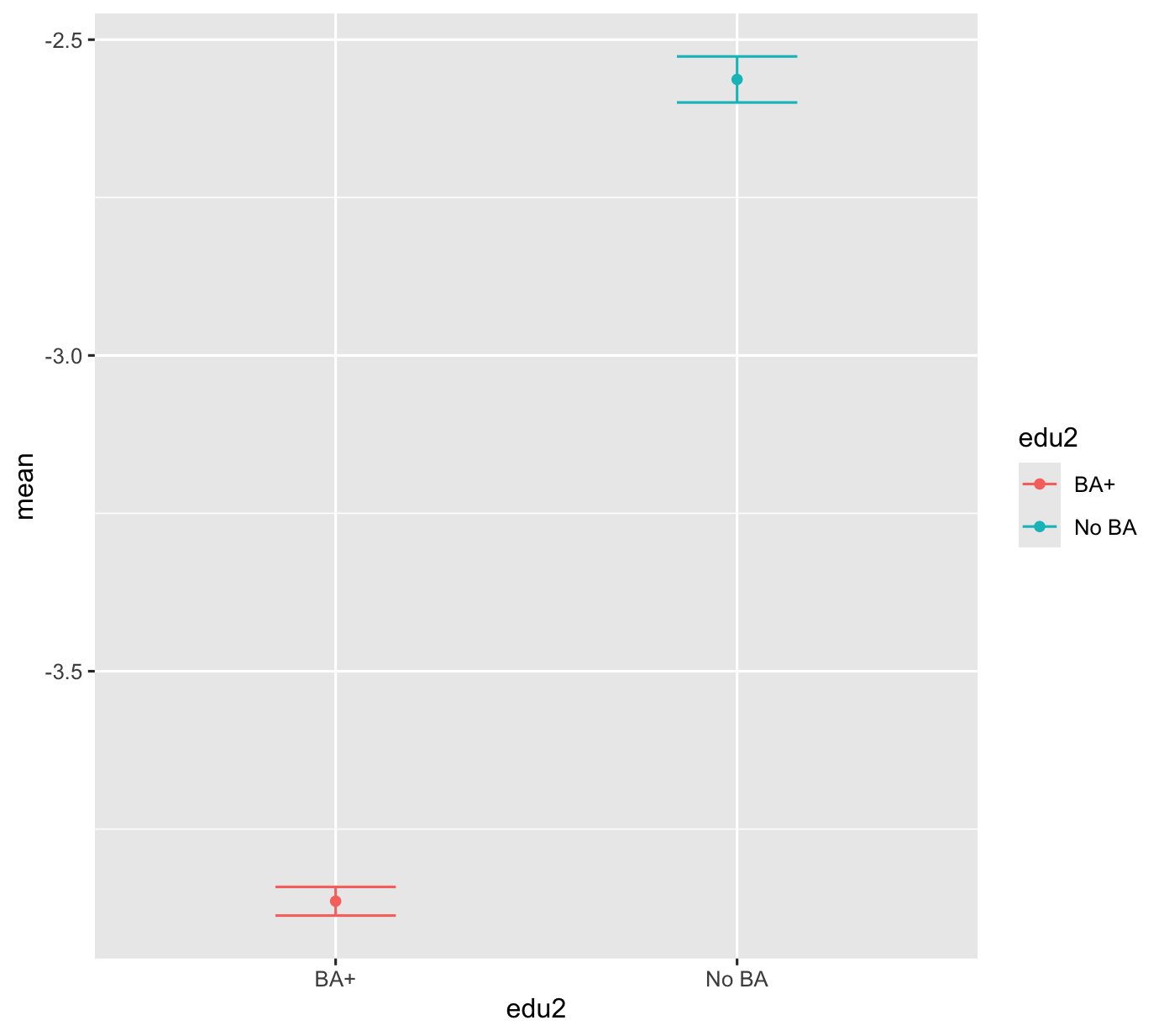
Age profile

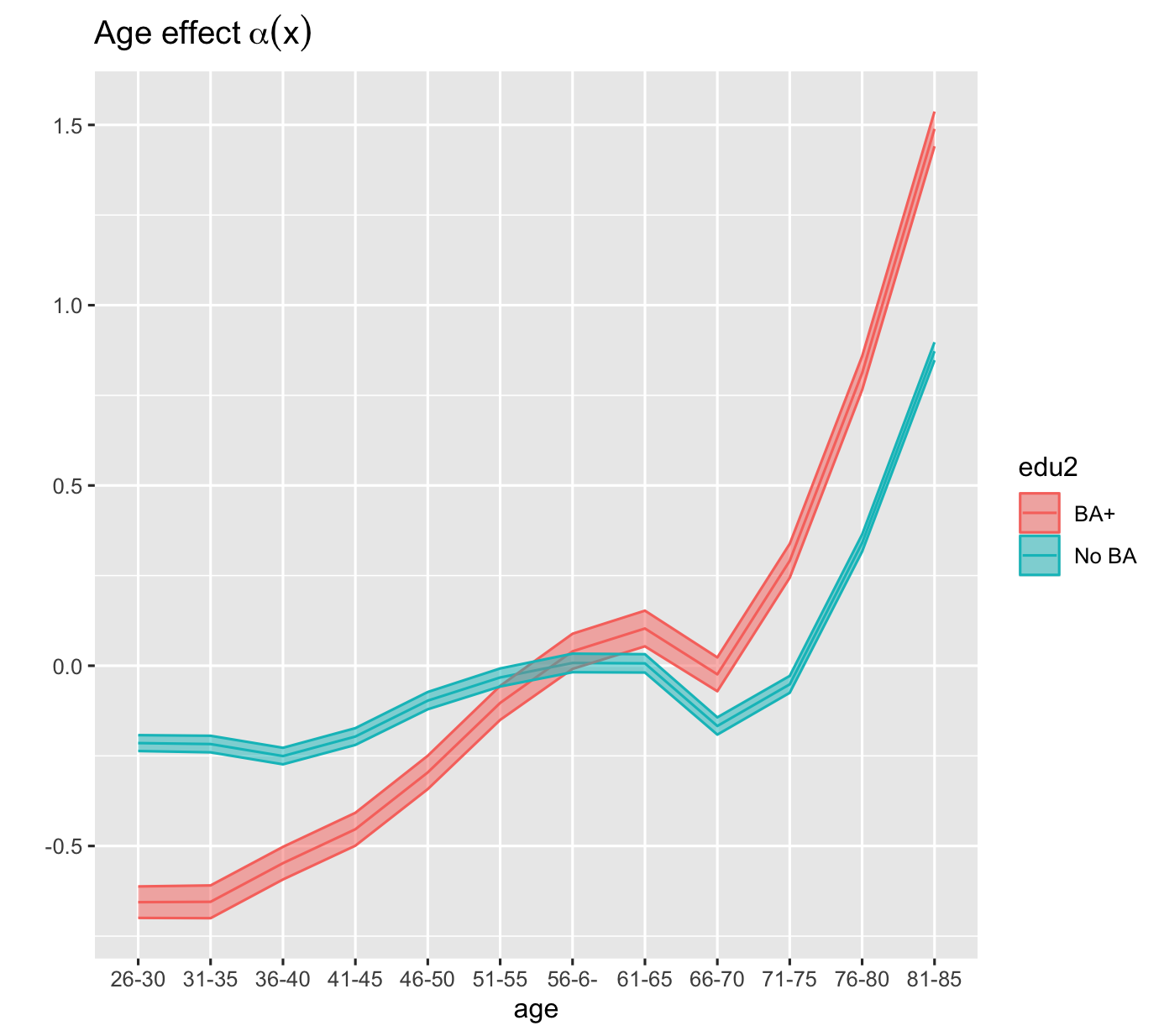
Results

Time trend

Age multiplier

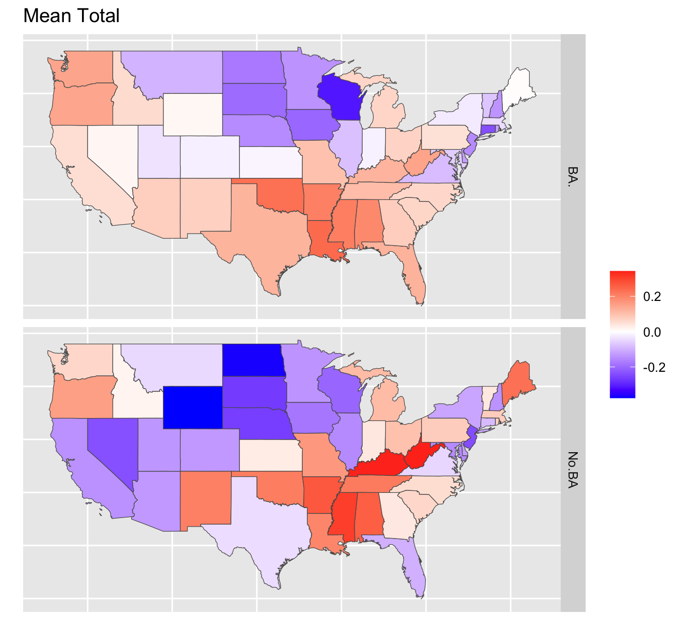
Results

State specific intercept

The way forward

• Include state specific trend
• Some of the estimated variances pf the FH estimator are zero…

Mortality in Italy

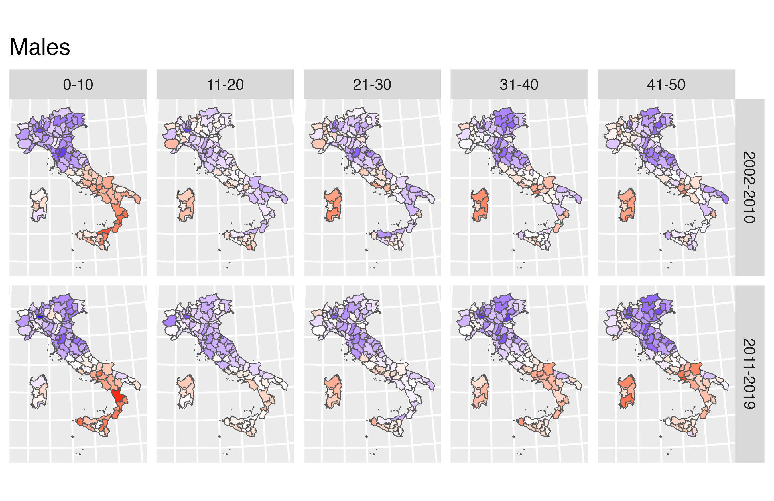
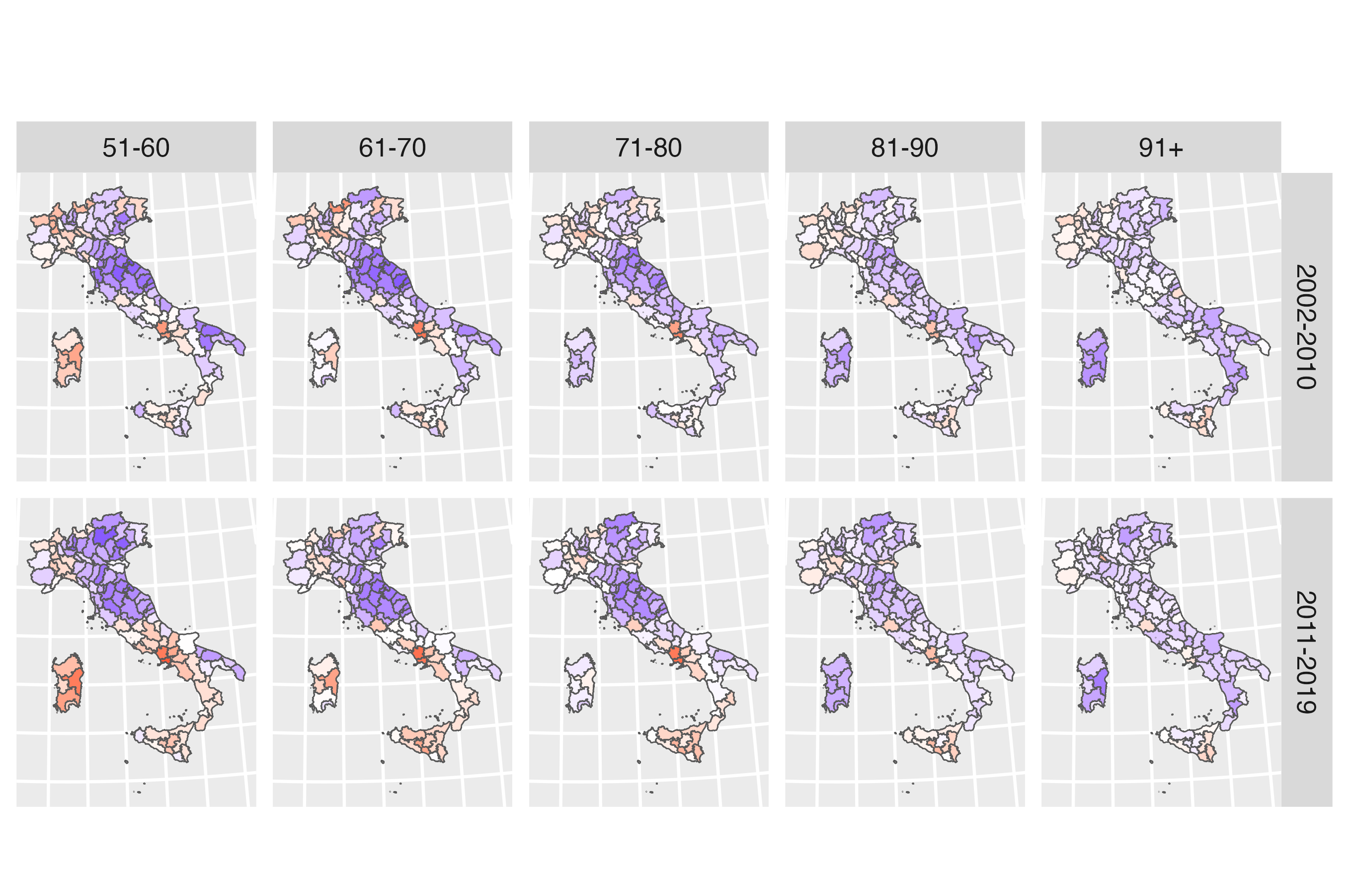
Italy as a case-study of mortality trends

1. Some of the lowest mortality levels in Europe: life expectancy of 83.4 in 2023.
2. Marked geographical differences, reflecting inequalities in wealth, educational level and employment opportunities.
3. Slowdown of mortality improvements since 2010.

---

Documented gendered geography of mortality in the second half of the 20th century – surprisingly little attention to the geography of mortality in the 21st century!

Data

ISTAT series of deaths and population counts:

• by single year of age
• separately by gender
• for each of the 107 Provinces
• for the period 1999-2019.

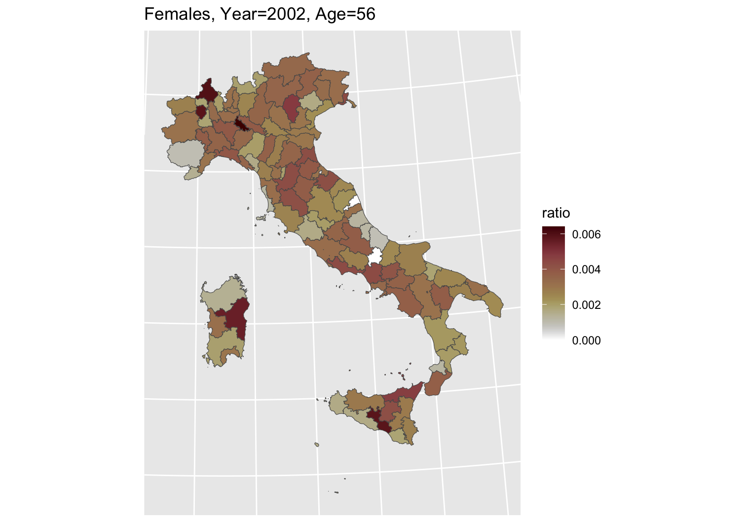
Good quality registers data – subject to random variability given the small size of the territorial units.

Research questions

The study contributes to understandings of geographical inequalities in mortality in the 21st century by asking:

1. How has gender- and age-specific mortality evolved over the last two decades?

2. How did mortality by age and gender vary at the provincial level?

3. And have geographical inequalities widened during the slowdown of survival improvement of the 2010s?

Model 1

Model 2

Model 1

We model males and females separately.

We assume the counts to be Poisson distributed \[ Y_{xts}|\lambda_{xts}\sim\text{Poisson}(E_{xts}e^{\lambda_{xts}}) \] with \[ \lambda_{xts} = \underbrace{\alpha_x + \beta_x\kappa_t + \epsilon_{xts}}_{1} + \underbrace{\omega_{sg_x}}_{2} \]

1. Traditional Lee-Carter model

2. Spatial effect: allowed to vary for 10 different age classe

• BYM2 model for each age class (replicate feature)

Model 2

\[ Y_{xts}|\lambda_{xts}\sim\text{Poisson}(E_{xts}e^{\lambda_{xts}}) \] with \[ \lambda_{xts} = \alpha_x + \beta_x\kappa_t + \omega_{s g_x p_t}+ \epsilon_{xts} \] with

\[ p_t = \left\{ \begin{aligned} 1 & \text{ for years 2002-2010}\\ 2 & \text{ for years 2011-2019}\\ \end{aligned} \right. \] This helps to capture different spatial trends in the two time periods.

1. How has gender- and age-specific mortality evolved over the last two decades?

Time effect

Age-specific multiplication factor

The graph on the left shows the estimated temporal trend. Mortality rates have been decreasing over time for both genders, but at a faster pace for men than for women. Against the overall declining pattern, we observe some evidence of a slowdown in the decline of mortality, particularly after 2012.

The graph on the right shows the estimated age-effect. The reduction of mortality rates has been more pronounced for younger age-classes than it is for individuals in their sixties and seventies.

2. How does mortality by age and gender vary at the provincial level?

The maps above show the estimates of mean mortality rates by age class, gender. Provinces in blu indicate lower than average mortality rates, and provinces in red indicate higher than average moratlity rates.

For both gender we observe a marked North/South divide for child mortality.

There is also evidence of geographical variation in mortality rates between age 30 and 80. for both gender. For women the disadvantage is mainly concentrated in the southern provinces of Campania Calabria and Sicilia, while for men it extends to the centre south.

After age 80, we observe comparatively (compared to younger ages) less variability across provinces for both gender – although we should highlight the existence of a Southern disadvantage for women but not for men.

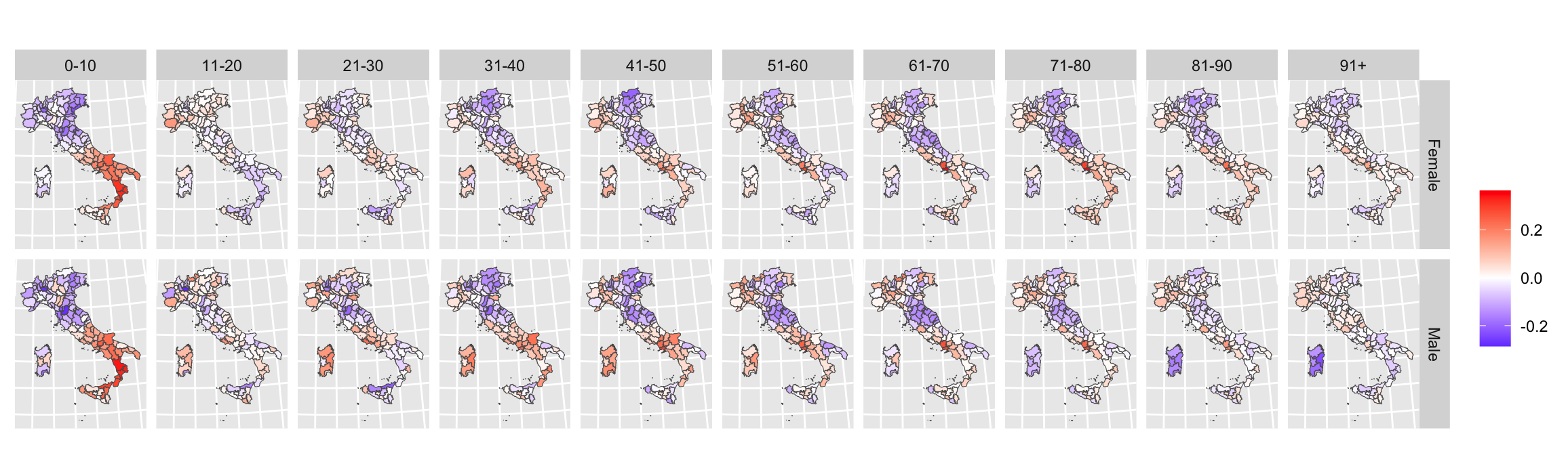
3. And have geographical inequalities widened during the slowdown of survival improvement of the 2010s?

Results for males.

Take home message

• varying geographical patterns depending on the combinations of age and gender considered
• geographical variability higher among younger adult men and among older adult women, suggesting the influence of age- and sex-specific, context-dependent, risk factors.
• widening of geographical inequalities between the first and second period

Conclusion

• Lee–Carter models provide a powerful framework to describe age-specific temporal dynamics. Many modern applications require extensions to account for spatial structure and complex data sources.

• inlabru extends the INLA framework to non-linear predictors, making it possible to easily fit Bayesian Lee–Carter models.

• Spatial extensions help uncover evolving local inequalities and changing regional patterns over time.